R/R Markdown Table Options for Multilevel Models
I am currently taking a multilevel modeling class in my PhD program. It is week 3-ish and I am learning a lot. The course is software-agnostic, meaning we can use any software we want (SPSS, SAS, Stata, R, HLM). The first assignment comes as a data set and Word document. I am working completely in R / R Markdown to generate both the data and model analyses and to complete the Word-based homework. Because I am working in an R -> Word workflow, I need to know what options I have for creating nice tables of my models.
So, I am taking a break from my first assignment to compare the default output of the most popular R model summary packages, look at some extended features, and make a cross-package comparison for my own future reference.
Let’s begin!
The Models
For this example, I am going to use Allison Horst’s palmerpenguins package for the data and produce two simple and non-substantive multi-level models. I will use lme4::lmer and lmerTest::lme4, which produces p-values and a few different estimates. Note: I will not be interpreting these models.
library(palmerpenguins)

# unconditional model
model_0 <- lme4::lmer(body_mass_g ~ 1 + (1 | island), REML = F, data=penguins)

model_0_lmertest <- lmerTest::lmer(body_mass_g ~ 1 + (1 | island), REML = F, data=penguins)

model_1 <- lme4::lmer(body_mass_g ~ sex + (1 | island), REML = F, data=penguins)

model_1_lmertest <- lmerTest::lmer(body_mass_g ~ sex + (1 | island), REML = F, data=penguins)
The Packages
The most popular packages that can take a model object and produce a neat table summary include modelsummary, gtsummary, huxtable, and sjPlot. I will generate default tables with each of these packages with the goal of being able to insert them into a Word document via knitr. I will try to keep customization to a minimum.
modelsummary
modelsummary offers the msummary function and allows me to create side-by-side tables. This will work for lme4 models, but will not work for lmerTest models unless you load the package broom.mixed first.
modelsummary::msummary(list(
  "Null Model" = model_0,
  "Model 1" = model_1))
| Null Model | Model 1 |
(Intercept) | 4048.143 | 3713.505 |
(275.116) | (273.909) | |
sd_(Intercept).island | 471.900 | 468.149 |
sd_Observation.Residual | 626.335 | 532.804 |
sexmale | 674.365 | |
(58.402) | ||
AIC | 5393.7 | 5147.3 |
BIC | 5405.2 | 5162.5 |
Log.Lik. | -2693.833 | -2569.644 |
Here, I have loaded broom.mixed and added a call for significance stars with stars=T.
library(broom.mixed)## Registered S3 methods overwritten by 'broom.mixed':
## method from
## augment.lme broom
## augment.merMod broom
## glance.lme broom
## glance.merMod broom
## glance.stanreg broom
## tidy.brmsfit broom
## tidy.gamlss broom
## tidy.lme broom
## tidy.merMod broom
## tidy.rjags broom
## tidy.stanfit broom
## tidy.stanreg broommodelsummary::msummary(list(
"Null Model" = model_0_lmertest,
"Model 1" = model_1_lmertest), stars = T)
| Null Model | Model 1 |
(Intercept) | 4048.143*** | 3713.505*** |
(275.116) | (273.909) | |
sd__(Intercept) | 471.900NA | 468.149NA |
sd__Observation | 626.335NA | 532.804NA |
sexmale | 674.365*** | |
(58.402) | ||
AIC | 5393.7 | 5147.3 |
BIC | 5405.2 | 5162.5 |
Log.Lik. | -2693.833 | -2569.644 |
* p < 0.1, ** p < 0.05, *** p < 0.01 | ||
Screenshot from Word
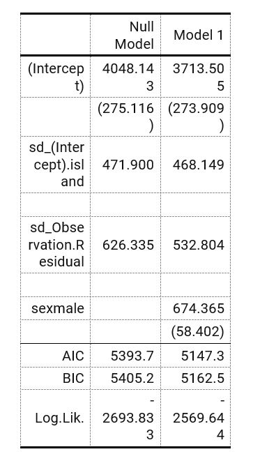
Screenshot from Word for msummary
Notes
msummaryproduces a decent side-by-side table in Word.- The default style looks like APA, which is something I would want.
- However, it splits the fixed effects of intercept and sex up so that intercept is above the random effects and sex is below.
- Finally, the default width is a bit narrow, meaning additional customization is needed. It can easily be customized using
flextable, which works well in Word. The following code coverts it toflextable:
modelsummary::msummary(list("Null Model" = model_0, "Model 1" = model_1), output = 'flextable')
gtsummary
gtsummary is based on the gt package, which allows easy and advanced customization of tables in R.
I could not get gtsummary to make a table for my null model, model_0. It produced the error: Error: must be a character vector, not a logical vector.. However, it worked for model_1 and model_1_lmertest. Here is the no frills default:
gtsummary::tbl_regression(model_1_lmertest)| Characteristic | Beta | 95% CI1 | p-value |
|---|---|---|---|
| sex | |||
| female | — | — | |
| male | 674 | 560, 789 | <0.001 |
|
1
CI = Confidence Interval
|
|||
That table is clearly not a good table. I did some googling, and found I had to add the following tidy function to produce a table with all estimates:
gtsummary::tbl_regression(model_1_lmertest, tidy_fun = broom.mixed::tidy)| Characteristic | Beta | 95% CI1 | p-value |
|---|---|---|---|
| sex | |||
| female | — | — | |
| male | 674 | 560, 789 | <0.001 |
| sd__(Intercept) | 468 | ||
| sd__Observation | 533 | ||
|
1
CI = Confidence Interval
|
|||
Screenshot from Word
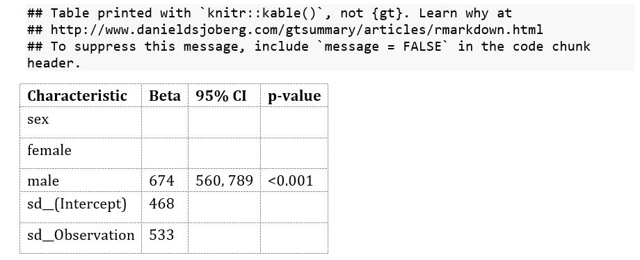
Screenshot from Word of gtsummary
Notes
- This table is created in
gt, but as of right now,gtdoesn’t work with Word so it was automatically converted to akabletable. - You can do a lot of customization using
gtand then convert it tokableorflextable(usingas_flex_table()). - While adding confidence intervals are nice, the lack of fit statistics makes the default output inadequate. Looking through the
gtsummaryreference, I do not see a way to add these. - Side-by-side tables requires saving each table as an object and then using
tbl_merge.
huxtable
huxtable works with both lme4 and lmerTest. It uses the huxreg function and can easily make side-by-side tables.
huxtable::huxreg(list(
                 "Null Model" = model_0_lmertest,
                 "Model 1" = model_1_lmertest))
## Warning in huxtable::huxreg(list(`Null Model` = model_0_lmertest, `Model 1` = model_1_lmertest)): Unrecognized statistics: r.squared
## Try setting `statistics` explicitly in the call to `huxreg()`| Null Model | Model 1 | |
| (Intercept) | 4048.143 *** | 3713.505 *** |
| (275.116) | (273.909) | |
| sd__(Intercept) | 471.900 | 468.149 |
| (NA) | (NA) | |
| sd__Observation | 626.335 | 532.804 |
| (NA) | (NA) | |
| sexmale | 674.365 *** | |
| (58.402) | ||
| N | 342 | 333 |
| logLik | -2693.833 | -2569.644 |
| AIC | 5393.665 | 5147.289 |
| *** p < 0.001; ** p < 0.01; * p < 0.05. | ||
Screenshot from Word
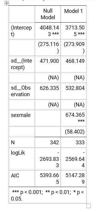
Screenshot from Word of huxtable
Notes
- By default
huxregproduces a nice side-by-side table. - The default looks like simple ASCII/Markdown table, but it knits to Word nicely without any need to make changes.
- Output looks like
modelsummary::msummarybut lacks ICC values. huxtablealso separates fixed effects likemodelsummary- Can be customized via
huxtableorflextableviaas_flextable- though I could not get this to work.
sjPlot
sjPlot is a table and visualization package meant for a number of social science methods (linear models, generalized linear models, PCA, robust standard errors, etc.).
Below is the HTML table. This table can be styled with CSS.
sjPlot::tab_model(model_0, model_1,
dv.labels = c("Null Model", "Model 1"))| Null Model | Model 1 | |||||
|---|---|---|---|---|---|---|
| Predictors | Estimates | CI | p | Estimates | CI | p |
| (Intercept) | 4048.14 | 3508.92 – 4587.36 | <0.001 | 3713.50 | 3176.65 – 4250.36 | <0.001 |
| sex [male] | 674.37 | 559.90 – 788.83 | <0.001 | |||
| Random Effects | ||||||
| σ2 | 392294.95 | 283879.82 | ||||
| τ00 | 222689.64 island | 219163.06 island | ||||
| ICC | 0.36 | 0.44 | ||||
| N | 3 island | 3 island | ||||
| Observations | 342 | 333 | ||||
| Marginal R2 / Conditional R2 | 0.000 / 0.362 | 0.185 / 0.540 | ||||
Screenshot from Word
NONE
Notes
- It works with
lmerTest. However, if you only uselme4,sjPlotautomatically adds p-values. sjPlotcreates a very nice table with random effects listed with their Greek values, \(\sigma^2\) and \(\tau\), plus ICC and \(R^2\)!- Unfortunately, it produces only an HTML table and this table cannot be automatically added to Word.
- Styling the table for HTML requires CSS.
- It cannot be converted to
flextableorkable
Final Thoughts
In a perfect world, we would be able to knit the sjPlot table to Word and be done with it. Unfortunately, this does not work for now. The best and easiest option would be using modelsummary::msummary. If you need p-values, use lmertest and broom.mixed, and be sure to call stars = T inside msummary. Then, make sure to also include output = 'flextable' to add more customization and allow your table to knit to Word.
The following example creates a simple function to automatically customize the table (useful if you will have multiple tables), and adds ICC and R2. I did not have time to organize the fixed and random effects, nor add the Greek symbols (ideally, in parentheses), but I think it’s easy to see how well modelsummary and flextable work together for your multilevel models!
library(tidyverse)
library(flextable)

#table formatting function
flex <- function(data, title=NULL) {
  set_table_properties(data, layout = "autofit", width = 1) %>%
  fontsize(size=12, part="all") %>%
      set_caption(title,
                  autonum = officer::run_autonum(seq_id = "tab",
                                                 pre_label = "Table ",
                                                 post_label = "\n",
                                                 bkm = "anytable"))
}

#adding ICC and R2 - note you can also write a function with glance_custom
# https://vincentarelbundock.github.io/modelsummary/articles/newmodels.html
mlm_added <- tribble(~term, ~"Null Model", ~"Model 1",
                     "ICC",
                        performance::icc(model_0)$ICC_conditional,
                        performance::icc(model_1)$ICC_conditional,
                     "pseudo R2",
          performance::r2(model_0)[["R2_conditional"]][["Conditional R2"]],
          performance::r2(model_1)[["R2_conditional"]][["Conditional R2"]])

#changing names of coefficients
cm <- c("sexmale"="Male",
        "sd__(Intercept)"="SD Intercept (τ00)",
        "sd__Observation" = "SD Observation (σ2)",
        "(Intercept)" = "Intercept")

#the final table
modelsummary::msummary(list("Null Model" = model_0,
                            "Model 1" = model_1),
                       output = 'flextable',
                       add_rows = mlm_added,
                       coef_map = cm) %>%
  flex("Multilevel Model of Palmer Penguins")
| Null Model | Model 1 |
Male | 674.365 | |
(58.402) | ||
SD Intercept (t00) | 471.900 | 468.149 |
SD Observation (s2) | 626.335 | 532.804 |
Intercept | 4048.143 | 3713.505 |
(275.116) | (273.909) | |
AIC | 5393.7 | 5147.3 |
BIC | 5405.2 | 5162.5 |
Log.Lik. | -2693.833 | -2569.644 |
ICC | 0.362 | 0.355 |
pseudo R2 | 0.362 | 0.540 |
Screenshot from Word
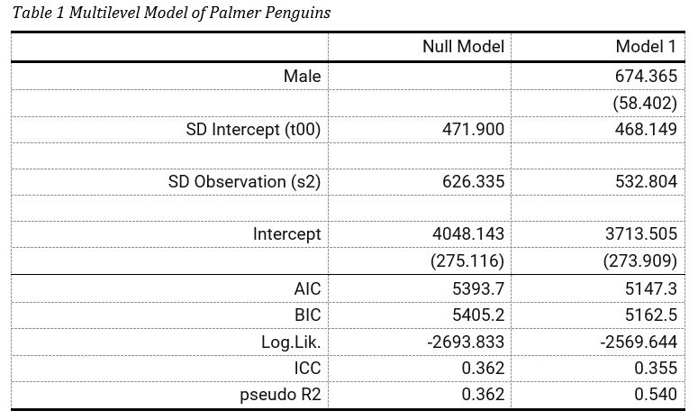
Screenshot from Word of Customized modelsummary
Do you know a better way to make great MLM tables in R Markdown, or have you figured out a sjPlot hack!? Please let me know.
Thanks to Vincet Arel-Bundock (https://twitter.com/VincentAB; author of modelsummary) for the tip about loading broom.mixed
Thanks to Daniel (https://twitter.com/strengejacke; author of sjPlot) for pointing out to use dv.labels
Anthony Schmidt
Data Scientist
My research interests include data science and education. I focus on statistics, research methods, data visualization, and machine learning.